Tuning SQL isn’t always easy, and it takes a lot of practice to recognise how any given query can be optimised. One of the most important slides of my
SQL training is the one summarising “how to be fast”:

Some of these bullets were already covered on this blog. For instance
avoiding needless, mandatory work, when client code runs queries or parts of queries that aren’t really necessary (e.g. selecting too many columns:
“needless”), but the database cannot
prove they’re needless, thus:
“mandatory” for the database to execute.
But as with many other performance related topics, one key message is not to guess, but to measure! Or, in other words, not to optimise prematurely, but to optimise actual problems.
SQL is full of myths
SQL is a
4GL (Fourth-generation programming language) and as such, has always been a cool, convenient way to express data related constraints and queries. But the declarative nature of the language also often meant that programmers are really looking into a crystal ball. A lot of people have blogged about a lot of half-true discoveries that might have been correct in some context and at some point of time (this blog is no exception).
For instance:
- Are correlated subqueries slower than their
LEFT JOIN equivalents?
- Are derived tables faster than views or common table expressions?
- Is
COUNT(*) faster than COUNT(1)?
Tons of myhts!
Measure your queries
To bust a myth, if you have good reasons to think that a differently written, but semantically equivalent query might be faster (on
your database), you should measure. Don’t even trust any execution plan, because ultimately, what really counts is the wall clock time in your production system.
If you can measure your queries in production, that’s perfect. But often, you cannot – but you don’t always have to. One way to compare two queries with each other is to benchmark them by executing each query hundreds or even thousands of times in a row.
As any technique, benchmarking has pros and cons. Here is a non-exhaustive list:
Pros
- Easy to do (see examples below)
- Easy to reproduce, also on different environments
- Easy to quickly get an idea in terms of orders of magnitude difference
Cons
- Not actually measuring productive situations (no one runs the same query thousands of times in a row, without any other queries in parallel)
- Queries may profit from unrealistic caching due to heavy repetition
- “Real query” might be dynamic, so the “same query” might really manifest itself in dozens of different productive queries
But if you’re fine with the cons above, the pros might outweigh, for instance, if you want to find out whether a correlated subquery is slower than its
LEFT JOIN equivalent
for a given query. Note my using italics here, because even if you find out it’s slower for
that given query it might be faster for other queries. Never jump to generalised rules before measuring again!
(More info and scripts about benchmarks here)
For instance, consider these two equivalent queries that run on the
Sakila database. Both versions try to find those actors whose last name starts with the letter A and counts their corresponding films:
LEFT JOIN
SELECT first_name, last_name, count(fa.actor_id) AS c
FROM actor a
LEFT JOIN film_actor fa
ON a.actor_id = fa.actor_id
WHERE last_name LIKE 'A%'
GROUP BY a.actor_id, first_name, last_name
ORDER BY c DESC
SELECT first_name, last_name, (
  SELECT count(*)
  FROM film_actor fa
  WHERE a.actor_id =
  fa.actor_id
) AS c
FROM actor a
WHERE last_name LIKE 'A%'
ORDER BY c DESC
The result is always:

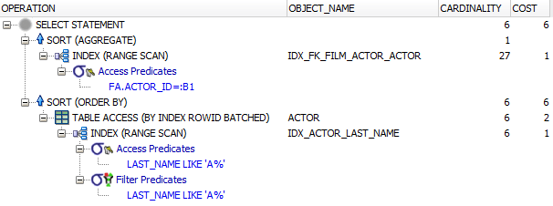
The queries have different execution plans on PostgreSQL, Oracle, SQL Server as can be seen below:
PostgreSQL LEFT JOIN

(Plan looks “better”)
PostgreSQL correlated subquery

(Plan looks “worse”)
Oracle LEFT JOIN

(Plan looks “more complicated”)
Oracle correlated subquery

(Plan looks “simpler”)
SQL Server LEFT JOIN

(Plan looks “reasonable”)
SQL Server correlated subquery
(Plan looks… geez, where’s my correlated subquery? It’s been transformed to a LEFT JOIN!)
Huh, as you can see, in SQL Server, both queries produce the exact same plan (as they should, because the queries are really equivalent). But not all databases recognise this and/or optimise this. At least, that’s what the estimated plans suggest.
Also, don’t jump to the conclusion that if the cost of one plan is lower then it’s a better plan than an alternative. Costs can only really be compared when comparing alternative plans
for the same query, e.g. in the Oracle example, we had both HASH JOIN and NESTED LOOP JOIN in a single plan, because Oracle 12c may collect runtime statistics and switch plans in flight thanks to the
Oracle 12c Adaptive Query Optimization features.
But let’s ignore all of this and look at actual execution times, instead:
Benchmarking the alternatives
As always, disclaimer: Some commercial databases do not allow for publishing benchmark results without prior written consent. As I never ask for permission, but always ask for forgiveness, I do not have consent, and I’m thus not publishing actual benchmark results.
I have anonymized the benchmark results by introducing hypothetical, non-comparable units of measurement, so you cannot see that PostgreSQL is totally slower than Oracle and/or SQL Server. And you cannot see that SQL Server’s procedural language is totally uglier than PostgreSQL’s and/or Oracle’s.
Legal people.
Solving problems we wouldn’t have without legal people, in the first place
Enough ranting. Some important considerations:
- Ideally, you’ll run benchmarks directly in the database using a procedural language, rather than, e.g. over JDBC to avoid network latency that incurs with JDBC calls, and other non-desired side-effects.
- Repeat the benchmarks several times to prevent warmup side-effects and other random issues, as your OS / file system may be busy with accidental Scala compilation, or Slack UI refreshes
- Be sure to actually consume the entire result set of each query in a loop, rather than just executing the query. Some databases may optimise for lazy cursor consumption (and possibly abortion). It would be unfair not to consume the entire result set
PostgreSQL
DO $$
DECLARE
  v_ts TIMESTAMP;
  v_repeat CONSTANT INT := 10000;
  rec RECORD;
BEGIN

  -- Repeat the whole benchmark several times to avoid warmup penalty
  FOR i IN 1..5 LOOP
    v_ts := clock_timestamp();

    FOR i IN 1..v_repeat LOOP
      FOR rec IN (
        SELECT first_name, last_name, count(fa.actor_id) AS c
        FROM actor a
        LEFT JOIN film_actor fa
        ON a.actor_id = fa.actor_id
        WHERE last_name LIKE 'A%'
        GROUP BY a.actor_id, first_name, last_name
        ORDER BY c DESC
      ) LOOP
        NULL;
      END LOOP;
    END LOOP;

    RAISE INFO 'Run %, Statement 1: %', i, (clock_timestamp() - v_ts);
    v_ts := clock_timestamp();

    FOR i IN 1..v_repeat LOOP
      FOR rec IN (
        SELECT first_name, last_name, (
          SELECT count(*)
          FROM film_actor fa
          WHERE a.actor_id =
          fa.actor_id
        ) AS c
        FROM actor a
        WHERE last_name LIKE 'A%'
        ORDER BY c DESC
      ) LOOP
        NULL;
      END LOOP;
    END LOOP;

    RAISE INFO 'Run %, Statement 2: %', i, (clock_timestamp() - v_ts);
  END LOOP;
END$$;
The result is:
INFO:  Run 1, Statement 1: 00:00:01.708257
INFO:  Run 1, Statement 2: 00:00:01.252012
INFO:  Run 2, Statement 1: 00:00:02.33151  -- Slack message received here
INFO:  Run 2, Statement 2: 00:00:01.064007
INFO:  Run 3, Statement 1: 00:00:01.638518
INFO:  Run 3, Statement 2: 00:00:01.149005
INFO:  Run 4, Statement 1: 00:00:01.670045
INFO:  Run 4, Statement 2: 00:00:01.230755
INFO:  Run 5, Statement 1: 00:00:01.81718
INFO:  Run 5, Statement 2: 00:00:01.166089
As you can see, in all 5 benchmark executions, the version with the correlated subquery seemed to have outperformed the version with the LEFT JOIN
in this case by roughly 60%! As this is PostgreSQL and open source, benchmark results are in actual seconds for 10000 query executions. Neat. Let’s move on to…
Oracle
SET SERVEROUTPUT ON
DECLARE
  v_ts TIMESTAMP WITH TIME ZONE;
  v_repeat CONSTANT NUMBER := 10000;
BEGIN

  -- Repeat the whole benchmark several times to avoid warmup penalty
  FOR r IN 1..5 LOOP
    v_ts := SYSTIMESTAMP;

    FOR i IN 1..v_repeat LOOP
      FOR rec IN (
        SELECT first_name, last_name, count(fa.actor_id) AS c
        FROM actor a
        LEFT JOIN film_actor fa
        ON a.actor_id = fa.actor_id
        WHERE last_name LIKE 'A%'
        GROUP BY a.actor_id, first_name, last_name
        ORDER BY c DESC
      ) LOOP
        NULL;
      END LOOP;
    END LOOP;

    dbms_output.put_line('Run ' || r || ', Statement 1 : ' || (SYSTIMESTAMP - v_ts));
    v_ts := SYSTIMESTAMP;

    FOR i IN 1..v_repeat LOOP
      FOR rec IN (
        SELECT first_name, last_name, (
          SELECT count(*)
          FROM film_actor fa
          WHERE a.actor_id =
          fa.actor_id
        ) AS c
        FROM actor a
        WHERE last_name LIKE 'A%'
        ORDER BY c DESC
      ) LOOP
        NULL;
      END LOOP;
    END LOOP;

    dbms_output.put_line('Run ' || r || ', Statement 2 : ' || (SYSTIMESTAMP - v_ts));
  END LOOP;
END;
/
Gee, check out the difference now (and remember, these are totally not seconds, but a
hypothetical unit of measurment, let’s call them Newtons. Or Larrys. Let’s call them Larrys
(great idea, Axel)):
Run 1, Statement 1 : 07.721731000
Run 1, Statement 2 : 00.622992000
Run 2, Statement 1 : 08.077535000
Run 2, Statement 2 : 00.666481000
Run 3, Statement 1 : 07.756182000
Run 3, Statement 2 : 00.640541000
Run 4, Statement 1 : 07.495021000
Run 4, Statement 2 : 00.731321000
Run 5, Statement 1 : 07.809564000
Run 5, Statement 2 : 00.632615000
Wow, the correlated subquery totally outperformed the LEFT JOIN query by an order of magnitude. This is totally insane. Now, check out…
SQL Server
… beautiful procedural language in SQL Server: Transact-SQL. With nice features like:
- Needing to cast INT values to VARCHAR when concatenating them.
- No indexed loop, only WHILE loop
- No implicit cursor loops (instead: DEALLOCATE!)
Oh well. It’s just for a benchmark. So here goes:
DECLARE @ts DATETIME;
DECLARE @repeat INT = 10000;
DECLARE @r INT;
DECLARE @i INT;
DECLARE @dummy1 VARCHAR;
DECLARE @dummy2 VARCHAR;
DECLARE @dummy3 INT;

DECLARE @s1 CURSOR;
DECLARE @s2 CURSOR;

SET @r = 0;
WHILE @r < 5
BEGIN
  SET @r = @r + 1

  SET @s1 = CURSOR FOR
    SELECT first_name, last_name, count(fa.actor_id) AS c
    FROM actor a
    LEFT JOIN film_actor fa
    ON a.actor_id = fa.actor_id
    WHERE last_name LIKE 'A%'
    GROUP BY a.actor_id, first_name, last_name
    ORDER BY c DESC

  SET @s2 = CURSOR FOR
    SELECT first_name, last_name, (
      SELECT count(*)
      FROM film_actor fa
      WHERE a.actor_id =
      fa.actor_id
    ) AS c
    FROM actor a
    WHERE last_name LIKE 'A%'
    ORDER BY c DESC

  SET @ts = current_timestamp;
  SET @i = 0;
  WHILE @i < @repeat
  BEGIN
    SET @i = @i + 1

    OPEN @s1;
    FETCH NEXT FROM @s1 INTO @dummy1, @dummy2, @dummy3;
    WHILE @@FETCH_STATUS = 0
    BEGIN
      FETCH NEXT FROM @s1 INTO @dummy1, @dummy2, @dummy3;
    END;

    CLOSE @s1;
  END;

  DEALLOCATE @s1;
  PRINT 'Run ' + CAST(@r AS VARCHAR) + ', Statement 1: ' + CAST(DATEDIFF(ms, @ts, current_timestamp) AS VARCHAR) + 'ms';

  SET @ts = current_timestamp;
  SET @i = 0;
  WHILE @i < @repeat
  BEGIN
    SET @i = @i + 1

    OPEN @s2;
    FETCH NEXT FROM @s2 INTO @dummy1, @dummy2, @dummy3;
    WHILE @@FETCH_STATUS = 0
    BEGIN
      FETCH NEXT FROM @s2 INTO @dummy1, @dummy2, @dummy3;
    END;

    CLOSE @s2;
  END;

  DEALLOCATE @s2;
  PRINT 'Run ' + CAST(@r AS VARCHAR) + ', Statement 2: ' + CAST(DATEDIFF(ms, @ts, current_timestamp) AS VARCHAR) + 'ms';
END;
And again, remember, these aren’t seconds. Really. They’re … Kilowatts. Yeah, let’s settle with kilowatts.
Run 1, Statement 1:  2626
Run 1, Statement 2: 20340
Run 2, Statement 1:  2450
Run 2, Statement 2: 17910
Run 3, Statement 1:  2706
Run 3, Statement 2: 18396
Run 4, Statement 1:  2696
Run 4, Statement 2: 19103
Run 5, Statement 1:  2716
Run 5, Statement 2: 20453
Oh my… Wait a second. Now suddenly, the correlated subquery is factor 5… more energy consuming (remember: kilowatts). Who would have thought?
Conclusion
This article won’t explain the differences in execution time between the different databases. There are a lot of reasons why a given execution plan will outperform another. There are also a lot of reasons why the same plan (at least what looks like the same plan) really isn’t because a plan is only a description of an algorithm. Each plan operation can still contain other operations that might still be different.
In summary, we can say that
in this case (I can’t stress this enough. This isn’t a general rule. It only explains what happens
in this case. Don’t create the next SQL myth!), the correlated subquery and the LEFT JOIN performed in the same order of magnitude on PostgreSQL (subquery being a bit faster), the correlated subquery
drastically outperformed the LEFT JOIN in Oracle, whereas the LEFT JOIN
drastically outperformed the correlated subquery in SQL Server (despite the plan having been the same!)
This means:
- Don’t trust your intitial judgment
- Don’t trust any historic blog posts saying A) is faster than B)
- Don’t trust execution plans
- Don’t trust this blog post here, because it is using uncomparable time scales (seconds vs newtons vs kilowatts)
- Don’t fully trust your own benchmarks, because you’re not measuring things as they happen in production
And sadly:
- Even for such a simple query, there’s no optimal query for all databases
(and I haven’t even included MySQL in the benchmarks)
BUT
by measuring two alternative, equivalent queries, you
may just get an idea what
might perform better for your system in case you do have a slow query somewhere. Perhaps this helps.
And now that you’re all hot on the subject, go book our
2 day SQL training, where we have tons of other interesting, myth busting content!
Like this:
Like Loading...
 The queries have different execution plans on PostgreSQL, Oracle, SQL Server as can be seen below:
PostgreSQL LEFT JOIN
The queries have different execution plans on PostgreSQL, Oracle, SQL Server as can be seen below:
PostgreSQL LEFT JOIN
 (Plan looks “better”)
PostgreSQL correlated subquery
(Plan looks “better”)
PostgreSQL correlated subquery
 (Plan looks “worse”)
Oracle LEFT JOIN
(Plan looks “worse”)
Oracle LEFT JOIN
 (Plan looks “more complicated”)
Oracle correlated subquery
(Plan looks “more complicated”)
Oracle correlated subquery
 (Plan looks “simpler”)
SQL Server LEFT JOIN
(Plan looks “simpler”)
SQL Server LEFT JOIN
 (Plan looks “reasonable”)
SQL Server correlated subquery
(Plan looks “reasonable”)
SQL Server correlated subquery
Small correction: Oracle performance units are called Larrys, not Newtons ;-)
You’re totally right. Fixed!
Your units are funny, but maybe you could keep it simpler by scaling all values so that the fastest (or slowest) result for a given database would be 1.0. If you don’t like the idea, then I’d recommend to use furlong per fortnight (you’re measuring speed, right?).
A small rant: Assuming there’s really such a thing like 4GL (starting in the seventies), then we should have 20GL by now, shouldn’t we?
I wonder how it comes that nearly no database “sees” that the queries are equivalent. I’d naively expect, such insight is a prerequisite for optimizations.
I did scale the results. There always is a result that is 1.0, I just didn’t display it. Furlong per fortnight sounds reasonable too, will remember for the next time.
Yeah, 4GLs should be a trivial thing compared to modern languages. We should all be asking Siri to compute things by now. But we aren’t.
There are many reasons why a database doesn’t “see” that the queries are equivalent. Mostly, transformations are omitted because each transformation (especially when cost based) adds a tremendous amount of complexity to the optimisation algorithm, which may already have a hard enough time to figure out the best order of joins.
In theory, all these transformations were known in the 70s. In practice, only recent computation power has allowed to actually explore many of them. Perhaps, machine learning will help an optimiser find a better path towards the best plan than costing statistics, though.
Can’t every nested query be replaced by a join? I don’t know, but if so, then it could be easiest to do it always so that the optimizer has don’t have to deal with the former at all.
The way it works now makes it hard for the programmer: There are different equivalent forms of the same query which leads to different timings depending on the RDBMS and also the current stats. So for the best speed, profiling is necessary, but not sufficient, as the plan may change later with changed stats or even a version upgrade.
The same holds for Java microoptimizations, but the microoptimizations are rarely important.
Does a database recognize a bad plan after it gets executed? It could get ashamed and try something else. ;)
I would say that probably (without fully proving it), a correlated subquery can always be replaced by a corresponding outer join, although sometimes, that transformation might be awfully complex. Also, the correlated subquery must not return more than one row, whereas a join may well do so, so the optimiser would make quite different choices as it wouldn’t know that the subquery returns at most one row…
And then: do note that the correlated subquery can outperform the join!
Yes, Oracle 11g knows adaptive cursor sharing (getting ashamed after a single bad execution) and Oracle 12c knows adaptive execution plans (getting ashamed while executing badly). SQL Server probably has something similar.
Also: Don’t get too upset about these differences. They hit me in a benchmark. They (probably) won’t hit you in production, mostly. A factor 5 performance difference is usually irrelevant for most operations because they’re sufficiently fast anyway…